This will be our first hands-on post, and we’re starting with a very visual type of attack that we can implement for free using services like Google Colab or in local environments with Anaconda/Miniconda, a Python virtual environment, Docker, or any other setup you’re more comfortable with.

Neural networks—specifically convolutional neural networks (CNNs)—are commonly used in computer vision tasks such as image classification, object detection, facial recognition, and more.

In this lab, however, we won’t be using a CNN. Instead, we’ll work with a fully connected neural network, which is more vulnerable to attacks like FGSM (Fast Gradient Sign Method). We’ll also use the MNIST (Modified National Institute of Standards and Technology) dataset of handwritten digits.

Our goal when training the neural network is to teach it to recognize handwritten digits. That means, when we show it one of these digits, it should be able to tell us what number it is—in other words, assign the correct label. To do that, the network needs to learn. Very simply put, the learning process looks like this:

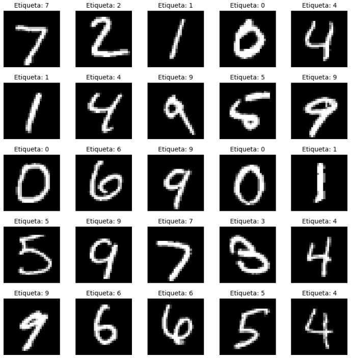
1. We start with thousands of images of handwritten digits (from 0 to 9). These digits come with labels, so we’ll tell the neural network what the correct answer is.
2. The neural network will go through the dataset several times (epochs), trying to predict which digit each image represents. At the beginning, it’ll make random guesses and will be initialized with weights that it will gradually adjust based on its mistakes. These weights determine how neurons in different layers are connected. Initially, weights are typically small random values, either positive or negative. It’s possible that if we train two identical networks but start with different initial weights, they might both learn well, reach different outcomes, or make different mistakes when facing attacks.
3. For each image, the network makes a prediction—for example, it might say the digit is a “6”.
4. We compare that prediction with the actual label—maybe we know it was a “4”.
5. We calculate the error. The more wrong the prediction is, the higher the error.
6. We inform the network of the mistake using a technique called backpropagation.
7. The network then adjusts its internal “connections” to try to make fewer mistakes next time. This is done by changing the weight values.

The way the network updates the weights isn’t random—it uses mathematical methods like gradient descent. A common analogy for explaining gradient descent is imagining you’re blindfolded on a mountain and trying to reach the lowest point. You can’t see, but you can feel the slope beneath your feet:

1. You sense which direction goes downhill
2. You take a small step that way, carefully 😉
3. You repeat this many times to walk down the mountain

Of course, this simple method doesn’t guarantee we’ll reach the lowest point of the entire mountain (global minimum)—we might get stuck in a small dip or valley instead (local minimum). But that’s a topic for another post.

In our example, we’ll use MNIST images of 28×28 pixels. Our network will flatten these into vectors of 784 (28×28) values. Then we’ll build a dense layer with 128 neurons, followed by a ReLU activation function, and finally an output layer with 10 neurons (one for each digit). That gives us 138 neurons (with weights) across 4 layers, including the flatten and ReLU layers. Our model will have a total of 101,770 trainable parameters:

• First dense layer: (784 × 128) + 128 biases = 100,480
• Second dense layer: (128 × 10) + 10 biases = 1,290

Why are we explaining all this about gradient descent? Because FGSM doesn’t try to reduce error—it tries to maximize it, doing the opposite of training. But instead of modifying the model’s weights, FGSM adds noise to the input images in a very specific way to trick the model. FGSM targets a trained model and slightly alters the input images to fool the model into making wrong predictions. In other words, if we take a handwritten “7”, it will subtly change the image in a way that increases the model’s error as much as possible, making it assign the wrong label with high confidence. To a human, it still looks like a “7”, but the model might say it’s a completely different digit.

FGSM is what we call a white-box attack, because the attacker knows everything about the model:

• The architecture
• The model’s weights
• The loss function
• The gradient calculation

In future posts, we’ll talk about black-box attacks, where the attacker can only send inputs to the model, observe the outputs, and hope to guess the right trick to fool it.

At the following link, you’ll find the notebook with the code we’ll use to train a model and run the FGSM attack. Let’s walk through some of the key parts of that code:

https://github.com/redteamailabs/ComputerVision/blob/main/FGSM_Practical_Fundamentals.ipynb

We define a simple neural network with 4 layers: one to flatten the image and turn it into a vector, a hidden layer with 128 neurons, a ReLU activation function, and an output layer with one neuron per digit. The forward method defines how data flows through the network.

class SimpleNN(nn.Module):
    def __init__(self):
        super(SimpleNN, self).__init__()
        self.fc = nn.Sequential(
            nn.Flatten(),
            nn.Linear(28*28, 128),
            nn.ReLU(),
            nn.Linear(128, 10)
        )

    def forward(self, x):
        return self.fc(x)

model = SimpleNN()

Then we train the model using the training set, a batch size of 64, and the Adam optimizer (Adaptive Moment Estimation, an improved version of classic gradient descent), along with cross-entropy loss, which is commonly used in classification tasks:

train_set = MNIST(root='./data', train=True, download=True, transform=transform)
train_loader = torch.utils.data.DataLoader(train_set, batch_size=64, shuffle=True)
optimizer = optim.Adam(model.parameters(), lr=0.001)
criterion = nn.CrossEntropyLoss()

We train the network only once (1 epoch): we compute predictions, calculate the loss, clear the gradients, perform backpropagation, and update the weights. We use a learning rate of 0.001, which is generally a good starting point. We’re training for just one epoch to keep execution fast, but we can increase the number of epochs to see the difference.

for epoch in range(1):  # Entrenamiento corto
    for images, labels in train_loader:
        outputs = model(images)
        loss = criterion(outputs, labels)
        optimizer.zero_grad()
        loss.backward()
        optimizer.step()

And we define the FGSM attack function, which takes the gradient of the loss with respect to the image and keeps only its sign. It multiplies this by an epsilon value that controls the strength of the attack—we can try different values to observe the effect. Finally, it adds this small perturbation to the original image:

def fgsm_attack(image, epsilon, data_grad):
    sign_data_grad = data_grad.sign()
    perturbed_image = image + epsilon * sign_data_grad
    return torch.clamp(perturbed_image, 0, 1)

We take a random image from the test set and calculate the gradient with respect to that image:

data_iter = iter(test_loader)
image, label = next(data_iter)
image.requires_grad = True

We ask the model to make a prediction about which digit it sees, and then we display it:

output = model(image)
init_pred = output.max(1, keepdim=True)[1]
print(f"Predicción original: {init_pred.item()} (correcta: {label.item()})")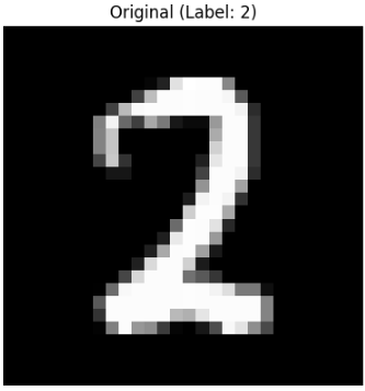

We calculate the loss and perform backpropagation to obtain the gradient of the error with respect to the image:

loss = criterion(output, label)
model.zero_grad()
loss.backward()
data_grad = image.grad.data

We generate the modified image by applying FGSM. Here, we can experiment with different epsilon values:

epsilon = 0.25
perturbed_image = fgsm_attack(image, epsilon, data_grad)

And we ask the model to make a prediction using the modified image, which will cause it to mislabel it:

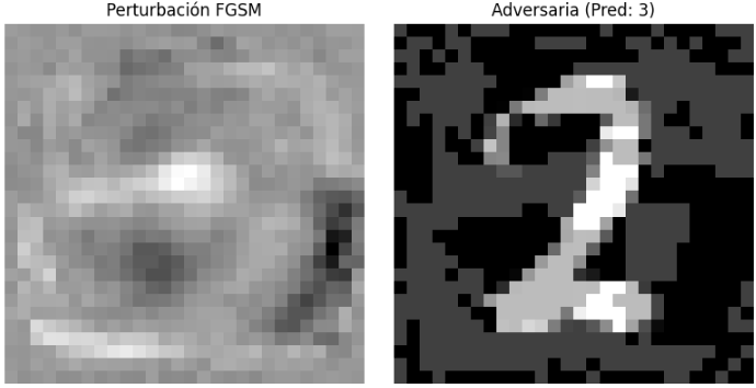
We still see a 2, but the model “sees” a 3.

In this case, we’ve used a very simple neural network. In future posts, we’ll move on to a convolutional neural network, which is more robust against this type of attack—though not invulnerable.