This post is a continuation of the previous one: “A Practical Introduction to FGSM.”

Here, we will focus on a Convolutional Neural Network. Convolutional Neural Networks (CNNs) represent one of the most significant breakthroughs in the field of artificial intelligence.

Their history began in 1998 when Yann LeCun introduced LeNet-5, the first successful CNN, used for handwritten digit recognition.

http://vision.stanford.edu/cs598_spring07/papers/Lecun98.pdf

However, the real turning point came in 2012 with AlexNet, developed by Alex Krizhevsky, which won the ImageNet competition with a staggering lead over traditional methods.

This victory marked the beginning of the deep learning revolution in computer vision.

https://papers.nips.cc/paper_files/paper/2012/file/c399862d3b9d6b76c8436e924a68c45b-Paper.pdf

CNNs are inspired by the visual cortex of mammals, where neurons respond to stimuli in specific regions of the visual field, known as receptive fields.

This architecture allows CNNs to capture hierarchical visual patterns, from simple edges to complex shapes and objects.

Convolutional Neural Networks, or CNNs, are a type of neural network specifically designed to work with data that has a grid-like structure, such as images. Unlike traditional neural networks, CNNs use convolutional operations to extract local features from the data, making them extremely effective in computer vision tasks. Some common applications include object recognition in images, image classification, and semantic segmentation. CNNs have revolutionized fields such as medicine, autonomous vehicles, and facial recognition.

Simple Neural Network (Fully Connected)
A simple neural network has no understanding that the image is a two-dimensional matrix. The first thing it does is flatten it into a vector of 784 values (28×28). From there, each of those pixels is connected to every neuron in the next layer.

This means the network doesn’t know which pixels are close to each other and cannot identify edges, corners, or shapes. Everything it learns is based on global correlations between numbers. It’s like trying to recognize a cat by looking at a list of brightness values, without knowing how they are arranged in the image.

Convolutional Network (CNN)
A CNN, on the other hand, respects the spatial structure of the image. It uses convolutional layers that apply small filters (kernels) sliding across the image to detect local patterns, such as edges, curves, or light and dark areas.

As the image passes through the layers, these filters combine simple patterns into more complex ones, allowing the network to understand key parts of the image: the shape of a “3,” the curve of a “5,” or the sharp angle of a “4.”

In this lab, we will train a CNN and also test it using FGSM.

https://github.com/redteamailabs/ComputerVision/blob/main/CNN_FGSM.ipynb

As always, we start by importing the necessary libraries:

import numpy as np
import tensorflow as tf
import matplotlib.pyplot as plt
from tensorflow.keras.datasets import mnist
from tensorflow.keras.models import Sequential
from tensorflow.keras.layers import Dense, Flatten, Conv2D, MaxPooling2D
from tensorflow.keras.optimizers import Adam

Import the required libraries:

• tensorflow and keras for neural networks,
• matplotlib to visualize images,
• numpy to work with arrays.

Next, we load and preprocess the data:

(x_train, y_train), (x_test, y_test) = mnist.load_data()
x_train = x_train / 255.0
x_test = x_test / 255.0
x_train = x_train.reshape(-1, 28, 28, 1)
x_test = x_test.reshape(-1, 28, 28, 1)

• Downloads the MNIST dataset.
• Normalizes the pixel values to the [0,1] range.
• Reshapes the images from (28, 28) to (28, 28, 1) so the model interprets them as grayscale images.

Define the CNN model:

def create_model():
model = Sequential([
Conv2D(32, (3, 3), activation='relu', input_shape=(28, 28, 1)),
MaxPooling2D((2, 2)),
Conv2D(64, (3, 3), activation='relu'),
MaxPooling2D((2, 2)),
Flatten(),
Dense(128, activation='relu'),
Dense(10, activation='softmax')
])
model.compile(optimizer=Adam(),
loss='sparse_categorical_crossentropy',
metrics=['accuracy'])
return model

• A simple convolutional network with 2 Conv2D layers, max-pooling, and dense layers.
• The model is compiled with Adam optimizer and cross entropy for multi-class classification.

Train the model:

model = create_model()
model.fit(x_train, y_train, epochs=5, batch_size=128, validation_split=0.1, verbose=1)

• The model is trained for 5 epochs using batches of 128 images.
• 10% of the data is held out for validation.

Generate the adversarial image using FGSM:

def create_adversarial_example_fgsm(model, image, label, epsilon=0.1):

This function generates an adversarial image from a real image.

• Converts the image to a tensor and enables gradient tracking with GradientTape.
• Computes the loss between the prediction and the true label.
• Calculates the gradient of the loss with respect to the input pixels.
• Takes the sign of the gradient and multiplies it by ε.
• Adds the perturbation to the original image.
• Uses clip_by_value() to keep the pixel values within the [0,1] range.

It returns a modified image that looks very similar to the original but is designed to fool the model.

Display the results:

def visualize_examples(model, index, epsilon):

• Picks an image from the test set.
• Generates an adversarial version using create_adversarial_example_fgsm().
• Makes predictions on both the original and the adversarial images.
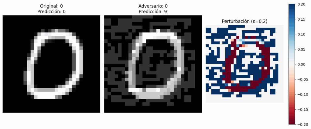
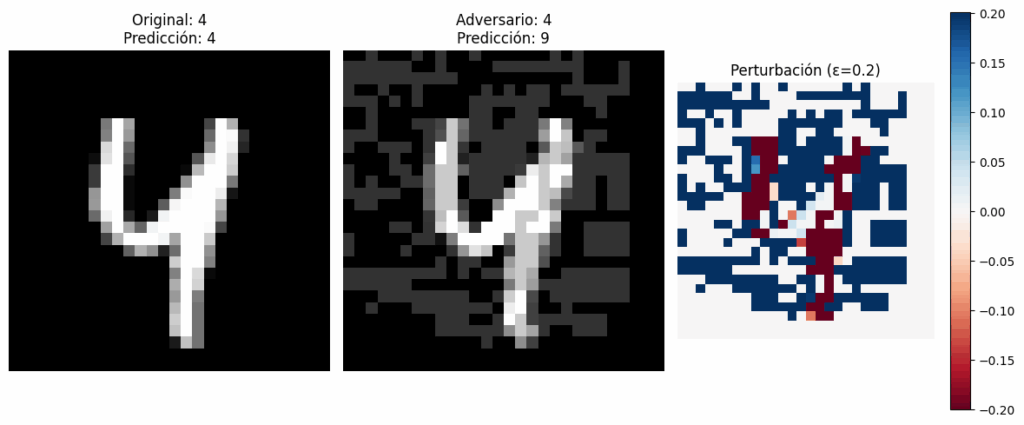
• Displays three images:
  1. Original image
  2. Adversarial image
  3. Applied perturbation (adversarial - original)

This lets you see whether the model gets fooled and what kind of distortion was introduced.

Run tests with several examples:

for idx in [10, 42, 56]:
for eps in [0.05, 0.1, 0.2]:
visualize_examples(model, idx, eps)

Generates and shows results for several test images with different ε values.

Evaluate the model’s robustness under attack:

def evaluate_under_attack(model, epsilon=0.1, num_examples=1000):

• Randomly selects num_examples from the test set.
• Generates adversarial versions of all of them.
• Evaluates the model on both original and adversarial data.
• Prints the accuracy on clean vs. adversarial images and the difference.

We confirm that model accuracy drops as attack intensity (ε) increases:

for eps in [0.01, 0.05, 0.1, 0.2, 0.3]:
evaluate_under_attack(model, epsilon=eps)

Although neither model is completely immune to the FGSM attack, the CNN shows greater robustness by default. Why?

• Because it learns local spatial patterns, not just isolated pixel correlations.
• Because the convolutional architecture introduces a degree of invariance to small perturbations, especially if they don’t affect key image regions.

However, both models can still be fooled by well-crafted perturbations if no defenses are applied.